Semantic Segmentation of Aerial Photographs

Abstract

Semantic segmentation of aerial imagery is a critical tool for applications such as environmental monitoring, urban planning, and disaster assessment. In this project, I employed the U-Net architecture attempting a variety of enhancements to improve segmentation accuracy on a set of satellite images of Mumbai. Seven models were trained and evaluated, each integrating specific changes to the base model in loss function, encoder depth, dropout regularization, and addition of attention mechanisms. Metrics including IoU, Dice, Precision, and Recall were used to assess model performance across six classes: vegetation, built-up areas, informal settlements, impervious surfaces, barren land, and water. A small “unclassified” class is also considered.

Introduction

Aerial photography has a wide variety of uses, including geology, archaeology, disaster assessment, and environmental monitoring (National Air and Space Museum, 2023). The technology improved and became more widely utilized for military purposes starting in World War I, and has since gone on to be used for tasks such as identifying different vegetation types, detecting diseased and damaged vegetation, and counting how many missiles, planes, and other military hardware adversaries have and where it is located (Baumann, 2014). Semantic segmentation, or pixel-wise classification, is useful in this context. Creating a mask that classifies all regions of an aerial image allows for monitoring of environmental conditions, foreign objects, and changing conditions over time. While this project explores semantic segmentation of aerial images, the technology is useful for a broad number of tasks in biology, robotics, agriculture, sports analysis, and more.

Semantic Segmentation Performance Metrics

Performance metrics for semantic segmentation can be thought of in terms of true positive (TP), false positive (FP), true negative (TN), and false negative (FN) classifications for each pixel.

The most common performance metric for semantic segmentation is the Jaccard Score, also known as Intersection over Union (IoU).

\[\mathrm{IoU} = \frac{\mathrm{TP}}{\mathrm{TP} + \mathrm{FP} + \mathrm{FN}}\]

Another frequently used metric for semantic segmentation is the Dice Score, also known as the F1 Score. This metric is formulated from two related metrics, Precision and Recall.

\[\mathrm{Precision} = \frac{\mathrm{TP}}{\mathrm{TP} + \mathrm{FP}}, \quad \mathrm{Recall} = \frac{\mathrm{TP}}{\mathrm{TP} + \mathrm{FN}}\] \[\mathrm{F1} = 2 \times \frac{\mathrm{Precision} \times \mathrm{Recall}}{\mathrm{Precision} + \mathrm{Recall}}\]

Intuitively, Precision can be interpreted as the proportion of predicted positive pixels that are correctly segmented, Recall as the proportion of ground truth pixels that are correctly segmented, and F1 as the harmonic mean of both.

Transposed Convolution

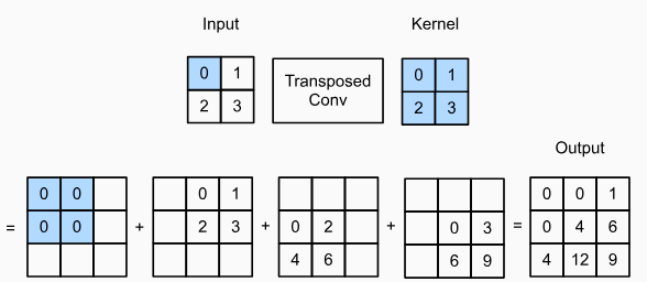
Transposed convolution, also known as upconvolution, is a method of upsampling similar to downsampling with convolution. Between each input pixel, zeros are inserted to increase the size of the feature map before convolution with the kernel. An example of transposed convolution is given below:

An Example Upconvolution with a 2×2 Input, 2×2 Kernel, and Stride of 1 (Zhang et al., 2023)

Dataset Description

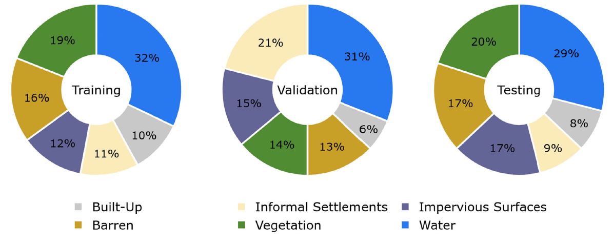
The dataset explored in this project is the Manually Annotated High Resolution Satellite Image Dataset of Mumbai for Semantic Segmentation (missing reference). The dataset was created from high-resolution, true-color satellite imagery of Pleiades-1A acquired on March 15, 2017 over Mumbai. There are six classifications: vegetation, built-up areas, informal settlements, impervious surfaces (roads, streets, parking lots, etc.), barren land, water, and a small number of unclassified pixels. The exact pixel distribution for the training set is given in Table 1.

Class	Informal Settlements	Built-Up	Impervious Surfaces	Vegetation	Barren	Water	Unclassified
# pixels	12,921,604	11,358,632	13,436,578	22,423,411	18,735,038	37,789,523	120,366

Table 1: Training Patch Pixel Distribution

Distribution of Labels Across Patches (Dabra & Kumar, 2023)

Methods

U-Net Architecture

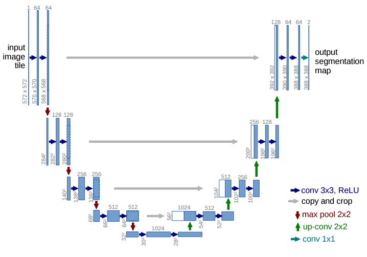
Ronneberger, Fischer, and Brox proposed the first U-Net architecture to segment cells in microscopic images (Ronneberger et al., 2015). The symmetric model consists of a contracting path, or encoder, on the left half and an expanding path, or decoder, on the right half. In the encoder, each level applies a $3\times 3$ convolution with ReLU activation before a $2\times 2$ max pooling operation is applied with stride 2 which reduces spatial dimensions by half. By doing this, the encoder is learning increasingly abstract representations of the original image while downsampling for computational efficiency. The decoder starts with the lowest spatial resolution, most abstract features and performs a series of $2\times 2$ upconvolutions which doubles the spatial dimensions. Importantly, a skip connection from the encoder of equivalent spatial dimension to each decoder layer is included to preserve spatial information lost during downsampling. The final output layer performs a $1\times 1$ convolution that reduces the number of channels to the number of classes.

The Original U-Net Architecture (Ronneberger et al., 2015)

Loss Functions

As with most classification networks, the output of our semantic segmentation model at each pixel is a vector of probabilities p, where each probability for class k is given by the softmax of the activations of each class input:

\[p_k(x, y) = \frac{\exp\bigl(a_k(x, y)\bigr)}{\sum_{k'=1}^{|k|} \exp\bigl(a_{k'}(x, y)\bigr)}\]

where $a_k(x,y)$ is the activation of class $k$ at pixel $(x,y)$ and $\lvert\mathbf{k}\rvert$ is the number of classes (in our case, 6). Then, $\mathbf{p}_k(x,y)$ can be interpreted as the probability that pixel $(x,y)$ belongs to class $k$.

Cross-Entropy

The most common loss function for semantic segmentation is pixel-wise cross-entropy, defined as

\[\mathcal{L}_{ce} = -\sum_{(x,y)} y(x,y)\,\log p(x,y)\]

where $\mathbf{y}(x,y)$ is a one-hot encoded vector of the true class of pixel $(x,y)$

Weighted Cross-Entropy

Real-world semantic segmentation datasets are often class-imbalanced, leading to issues with basic cross-entropy loss wherein the network is biased toward majority classes. To combat this, class-specific weights are often introduced to the loss function, often derived from the original data statistics (Csurka et al., 2023). Such a cost-sensitive loss function can be seen in the original proposal where the authors introduce a weighting function for each pixel that both balanced the classes and emphasized learning separation borders between cells (Ronneberger et al., 2015). Here, the loss function is of the form

\[\mathcal{L}_{wce} = -\sum_{(x,y)} w(x,y)\;y(x,y)\,\log p(x,y)\]

where $w$ is a pre-computed function of $(x,y)$.

Focal Loss

Focal loss includes a focusing parameter $\gamma$ which controls the down-weighting of well-classified pixels, designed to handle class imbalance and prioritize difficult samples with dice loss for improved segmentation overlap.

\[\mathcal{L}_{wfl} = -\sum_{(x,y)}\sum_{c=1}^{\lvert k \rvert} w_c\,(1 - p_c(x,y))^\gamma\,y_c(x,y)\,\log p_c(x,y)\]

Data Augmentation

The image patches are first upsampled to a resolution of $128\times 128$ to ensure they are compatible with the chosen network architecture, which involves a series of convolutional and pooling operations. This particular size is important because the network utilizes skip-connections between the encoder and decoder layers, and it includes five sequential downsampling stages. Each downsampling stage reduces both the height and width of the input by a factor of two, and since $2^5 = 32$, the input dimensions must be multiples of 32 to avoid boundary issues or the need for cropping. By setting the image patches to $128\times 128$, we ensure smooth downsampling at every stage, maintaining feature alignment between the encoder and decoder pathways for effective information transfer.

To further enhance the training process and reduce the risk of overfitting, at the start of each training epoch, the original image patch and its associated mask are randomly rotated by a multiple of $90^\circ$. This approach adds rotational invariance to the model’s learned features and expands the effective size of the training dataset, helping the network generalize better to novel samples and preventing it from simply memorizing the training images.

Model Selection

Pre-trained models from the Segmentation Models PyTorch library (Iakubovskii, 2019) were used. EfficientNet-B0 (Tan & Le, 2020) pre-trained on ImageNet (missing reference) was chosen as the encoder for its small size (4M parameters), reducing overfitting and accommodating limited compute resources.

Optimizer & Scheduler

The Adam optimizer was used with an initial learning rate of $1\times 10^{-4}$ (Dabra & Kumar, 2023). A LambdaLR scheduler decayed the learning rate by a factor of 0.1 every 40 epochs:

\[\lambda(\text{epoch}) = 0.1^{\frac{\text{epoch}}{40}}\]

This scheduler systematically reduces the learning rate as training progresses, implementing an exponential decay strategy. Such a decay is beneficial for fine-tuning as it allows the model to make large updates during the initial phases of training when significant adjustments are needed, and smaller, more precise updates in later stages to refine the learned features.

Early Stopping

To mitigate the risks of overfitting and the excessive consumption of computational resources during model training, we incorporate an early stopping mechanism in our training pipeline. Early stopping serves as a regularization technique by monitoring the model’s performance on a separate validation dataset and halting the training process when no significant improvement is observed over a predefined number of epochs. Specifically, in my implementation, we track the validation loss at each training epoch and terminate the training if the validation loss does not decrease for five consecutive epochs.

Results

Model 1

The initial model follows the Methods exactly and serves as a baseline.

Model 1 Training

Model 1 Predictions

Model 2

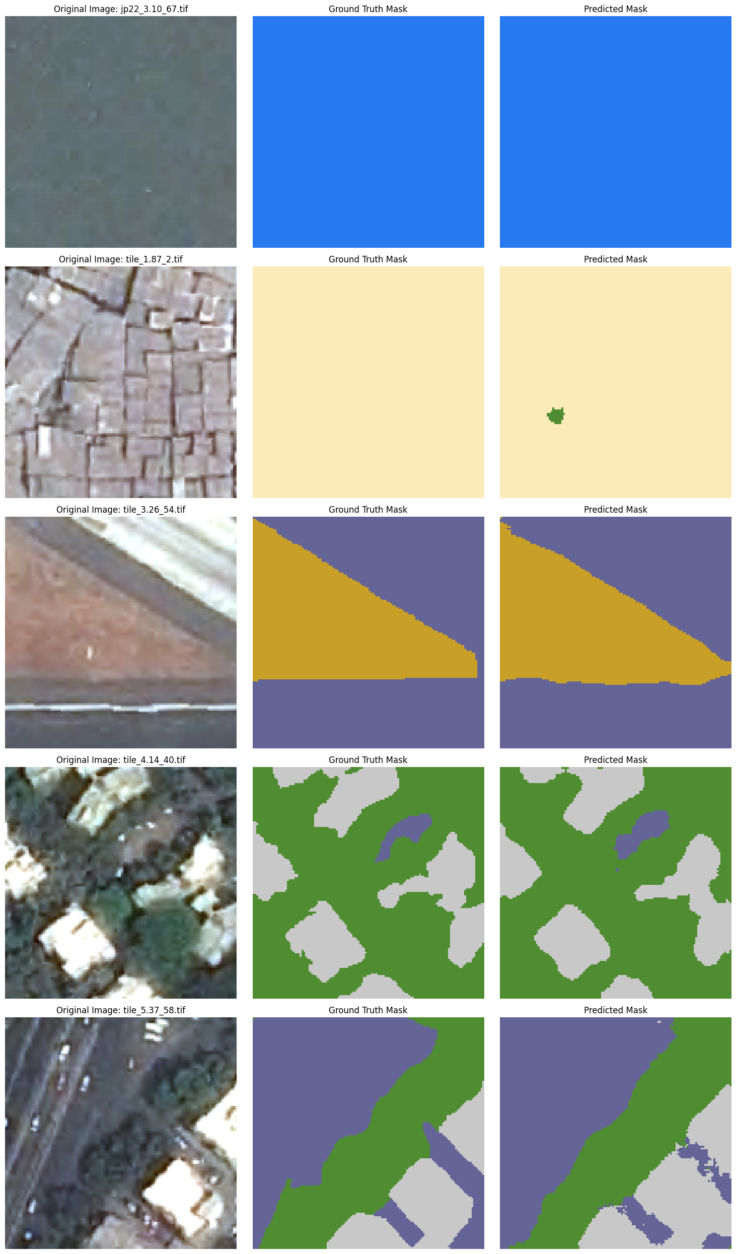
This model introduces Dice loss alongside cross-entropy to better address class imbalance by directly optimizing overlap between prediction and ground truth.

Model 2 Predictions

Model 3

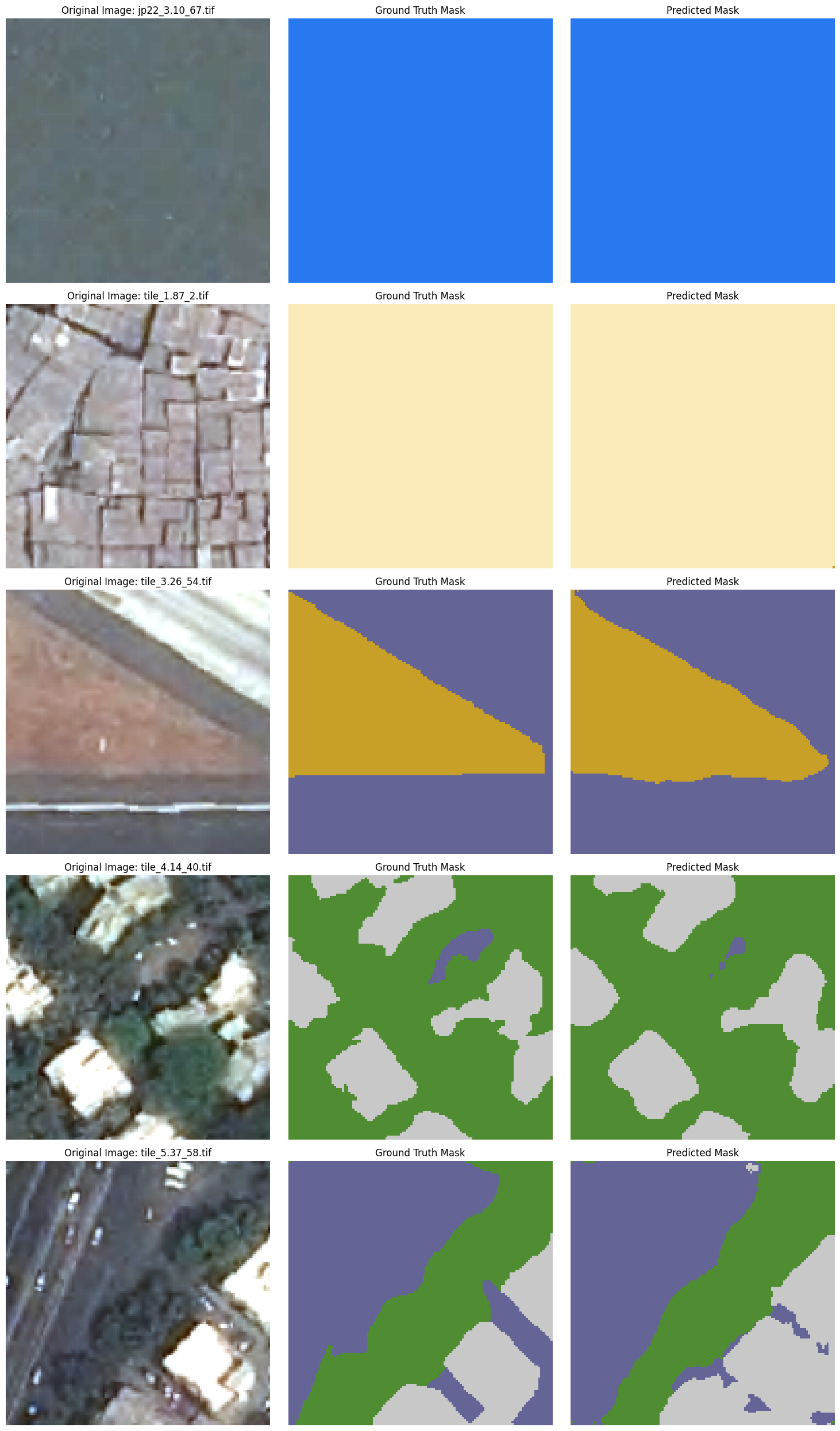
Class-weighted cross-entropy is combined with Dice loss. Weights were computed as the inverse class frequency and normalized; the unclassified class was scaled down by 0.001 before normalization.

Model 3 Predictions

Model 4

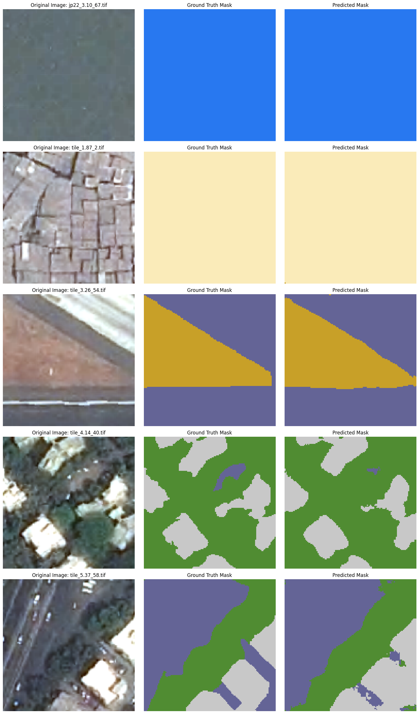
A shallower U-Net (encoder depth 4, decoder channels [256,128,64,32]) reduces compute overhead while maintaining performance.

Model 4 Predictions

Model 5

Dropout (p=0.2) was added in the decoder to improve generalization by reducing overfitting.

Model 5 Predictions

Model 6

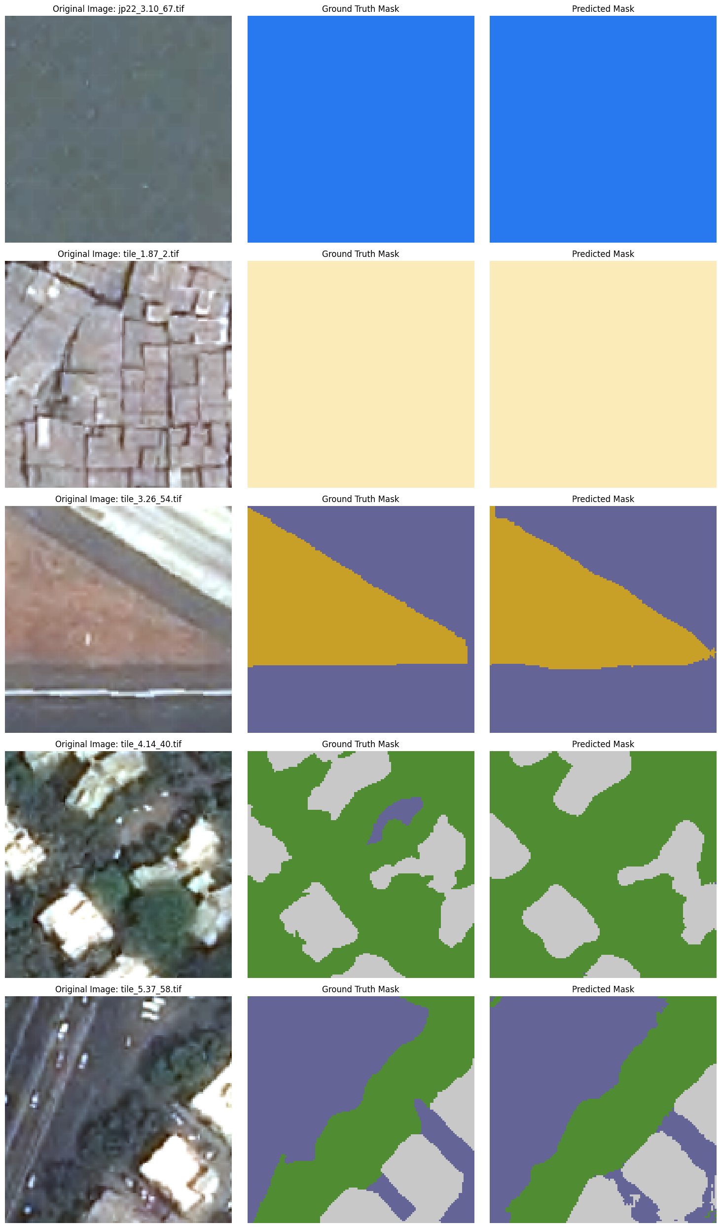
SCSE attention blocks were incorporated in the decoder to recalibrate feature channels and focus on important regions (Roy et al., 2018). SCSE blocks recalibrate feature responses by adaptively weighting each channel through a squeeze operation (global average pooling) followed by an excitation step using fully connected layers and sigmoid activation. This mechanism allows the network to emphasize important features while suppressing irrelevant ones, enhancing the model’s focus on key regions of the feature maps.

Model 6 Predictions

Model 7

Combines SCSE attention, weighted focal loss, Dice loss, AdamW optimizer, and a cosine annealing scheduler with warm restarts for refined performance.

Model 7 Training

Model 7 Predictions

Model Comparison

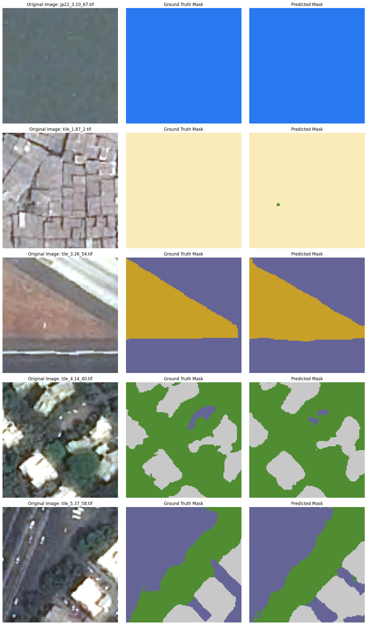
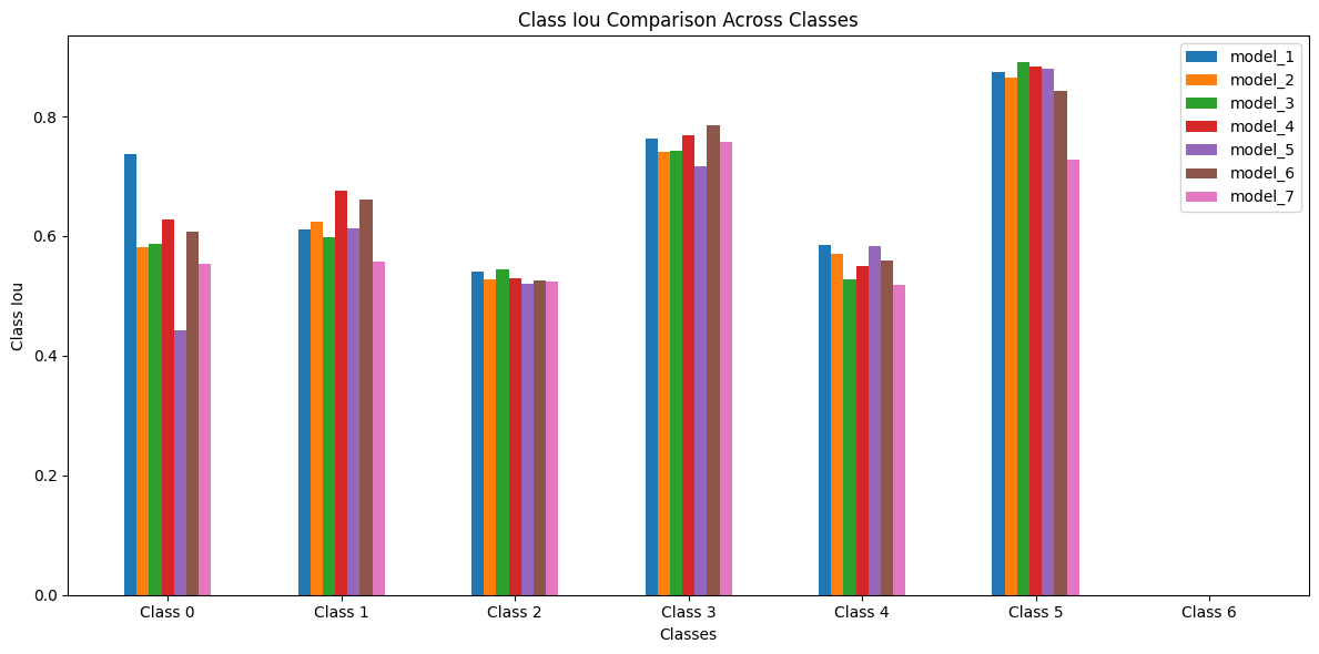
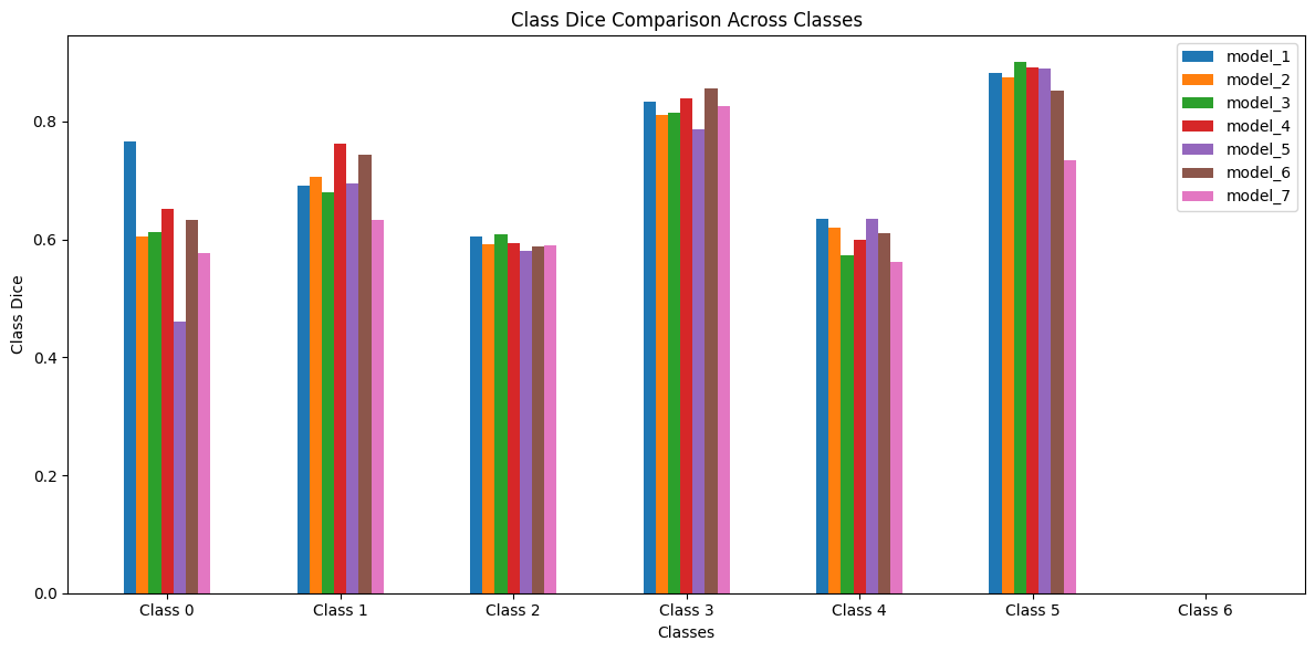
Model 1 stands out as the best-performing model overall. It consistently achieves the highest Dice and IoU scores for critical classes, while maintaining strong performance across other classes. Model 4 closely follows, excelling particularly in Class 1 and Class 3, where it outperforms other models. Model 6 also demonstrates strong performance, particularly in Class 3 and Class 5, where its inclusion of SCSE attention blocks helps improve feature focus and segmentation quality. While it falls slightly behind Models 1 and 4 in certain classes, it remains a reliable model with strong average Dice and IoU scores. On the other hand, Model 2 and Model 7 underperform.

Overall Comparison

Class-Wise IoU Comparison

Class-Wise Dice Comparison

Conclusion

This work highlights the strengths and trade-offs of various modifications to the U-Net architecture for aerial image segmentation. Model 1, despite being the most basic, was the highest-performing model across all evaluation metrics. Model 4 demonstrates that computational efficiency can be achieved without substantial loss in accuracy. Model 6 showcases the value of attention mechanisms for complex regions. However, limitations remain in capturing fine boundaries and in class imbalance. A simple improvement may be to use an ensemble of U-Nets (Marmanis et al., 2016).

Future Work

While this project showed promising results, improvements can certainly be made. The models seemed to struggle with fine-detailed class boundaries, for example, a jagged settlement bordering a patch of vegetation. To enhance the precision of these boundaries, future work could explore incorporating higher-resolution input data, which would provide more detailed information for the model to learn from. Additionally, implementing multi-scale feature extraction techniques, such as feature pyramids, could help the model capture both global and local context more effectively. Another promising approach is the integration of Conditional Random Fields as a post-processing step to refine segmentation edges by considering spatial dependencies and contextual relationships between pixels. Employing these methods could lead to smoother and more accurate delineations of classes with intricate boundaries and improve overall segmentation performance.

Class imbalance proved to be an issue throughout the project, with classes like water dominating the optimization problem. While class-balancing was attempted through loss function weighting, more methods exist to address this challenge. Future work could investigate advanced strategies such as Synthetic Minority Over-sampling Technique (SMOTE) to generate synthetic samples for underrepresented classes, thereby increasing their presence in the training dataset. Another potential approach is the use of data augmentation techniques such as geometric transformations or color jittering to artificially enhance the diversity and quantity of these classes. Exploring these methods could lead to a more balanced training process and improve the model’s ability to accurately segment all classes.

I chose a relatively basic encoder given time and compute constraints, but more advanced encoders such as ResNet or Vision Transformers (ViT) could be integrated to enhance feature extraction capabilities. Vision Transformers, which leverage self-attention mechanisms to capture long-range dependencies within the image, might enable the model to better understand complex spatial relationships, leading to more accurate semantic segmentation.

Finally, it would be useful to explore other state-of-the-art models for semantic segmentation beyond the U-Net. Architectures such as DeepLabv3+, PSPNet, and Mask R-CNN offer alternative approaches that incorporate advanced techniques like atrous convolutions, pyramid pooling modules, and instance segmentation capabilities. For example, DeepLabv3+ utilizes atrous spatial pyramid pooling to capture multi-scale contextual information, which can improve the segmentation of objects at different sizes. PSPNet’s pyramid pooling module effectively aggregates global and local context, enhancing the model’s ability to understand complex scenes. Mask R-CNN extends the capabilities of object detection frameworks to perform instance segmentation, allowing for more precise delineation of objects within an image.

References

2023
- The Beginnings and Basics of Aerial PhotographyJul 2023Accessed: Dec. 8, 2024
- Dive into Deep LearningJul 2023
- Evaluating green cover and open spaces in informal settlements of Mumbai using deep learningNeural Computing and Applications, Jul 2023
- Semantic Image Segmentation: Two Decades of ResearchJul 2023
2020
- EfficientNet: Rethinking Model Scaling for Convolutional Neural NetworksJul 2020
2019
- Segmentation Models PytorchJul 2019
2018
- Recalibrating Fully Convolutional Networks with Spatial and Channel ’Squeeze & Excitation’ BlocksJul 2018
2016
- Semantic Segmentation of Aerial Images with an Ensemble of CNNsISPRS Annals of Photogrammetry, Remote Sensing and Spatial Information Sciences, Jul 2016
2015
- U-Net: Convolutional Networks for Biomedical Image SegmentationJul 2015
2014
- HISTORY OF REMOTE SENSING, AERIAL PHOTOGRAPHYJul 2014Accessed: Dec. 8, 2024